What is a power query?

Power query is essentially a technology you can use within Excel to connect datasets together within an Excel spreadsheet. You can use power query to pull data from a range of sources, including webpages, databases, other spreadsheets, and multiple file types.

Once the data is imported, you can also use the power query editor to clean and transform the data. Finally, you can import the transformed data into your existing spreadsheet.

Common actions you can use in the power query editor after importing data include filtering, removing duplicates, splitting columns, formatting data, and merging data.

The core benefit is that tasks that would take you hours to do manually can be performed in minutes with power query. Plus, you can repeatedly use the same cleaning or transformation actions again at the click of a button when the data sources are updated.

How to Use Power Queries in Excel

When learning how to use something like power query, the most useful method is with an example. The steps below can be applied to any type of data set, and the functionalities highlighted can be replaced with other ways to use queries as needed.

In this example, I’m pulling together sales data from two different geographic regions for analysis. The data comes from the U.S. and the U.K., with formatting and currencies that are written differently and formatted differently across two spreadsheets.

My goal is to combine these data sets in one sheet, with the data cleaned and easily interpreted and analyzed in one place.

Step 1. Open Excel and access power query.

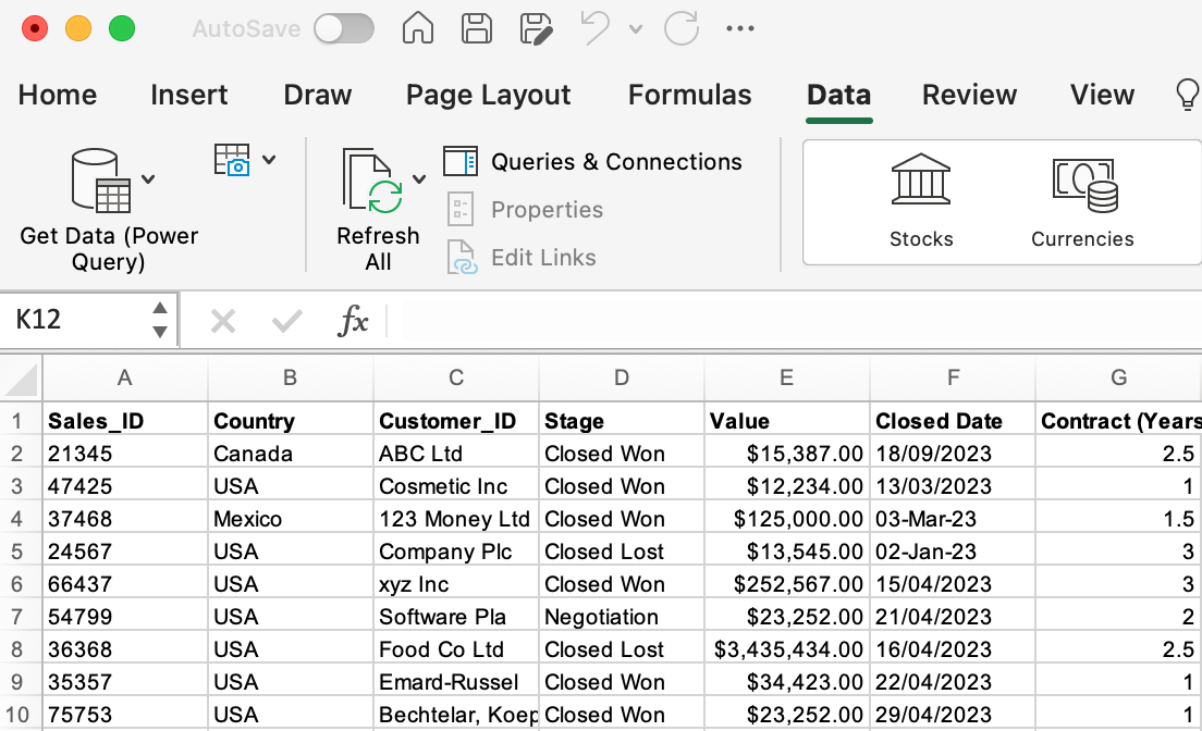
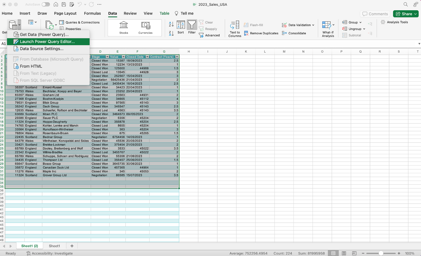
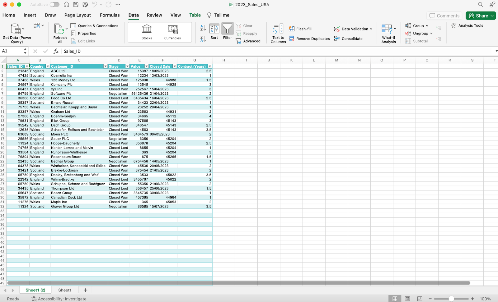
First things first, open the main spreadsheet you’ll be working from. In this case, I’ve opened my USA sales spreadsheet, as this is where I want to clean and combine data.

In the main ribbon, click on “Data.” You’ll see “Get Data (Power Query)” as the first item in the Data ribbon.

Step 2. Import your data.

Click on the dropdown to access your power query options.

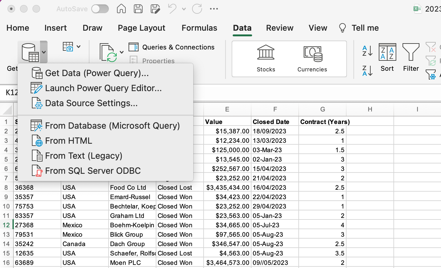
In this first step, we want to hit “Get Data,” so we can start a query using the data in the U.K. sales spreadsheet.

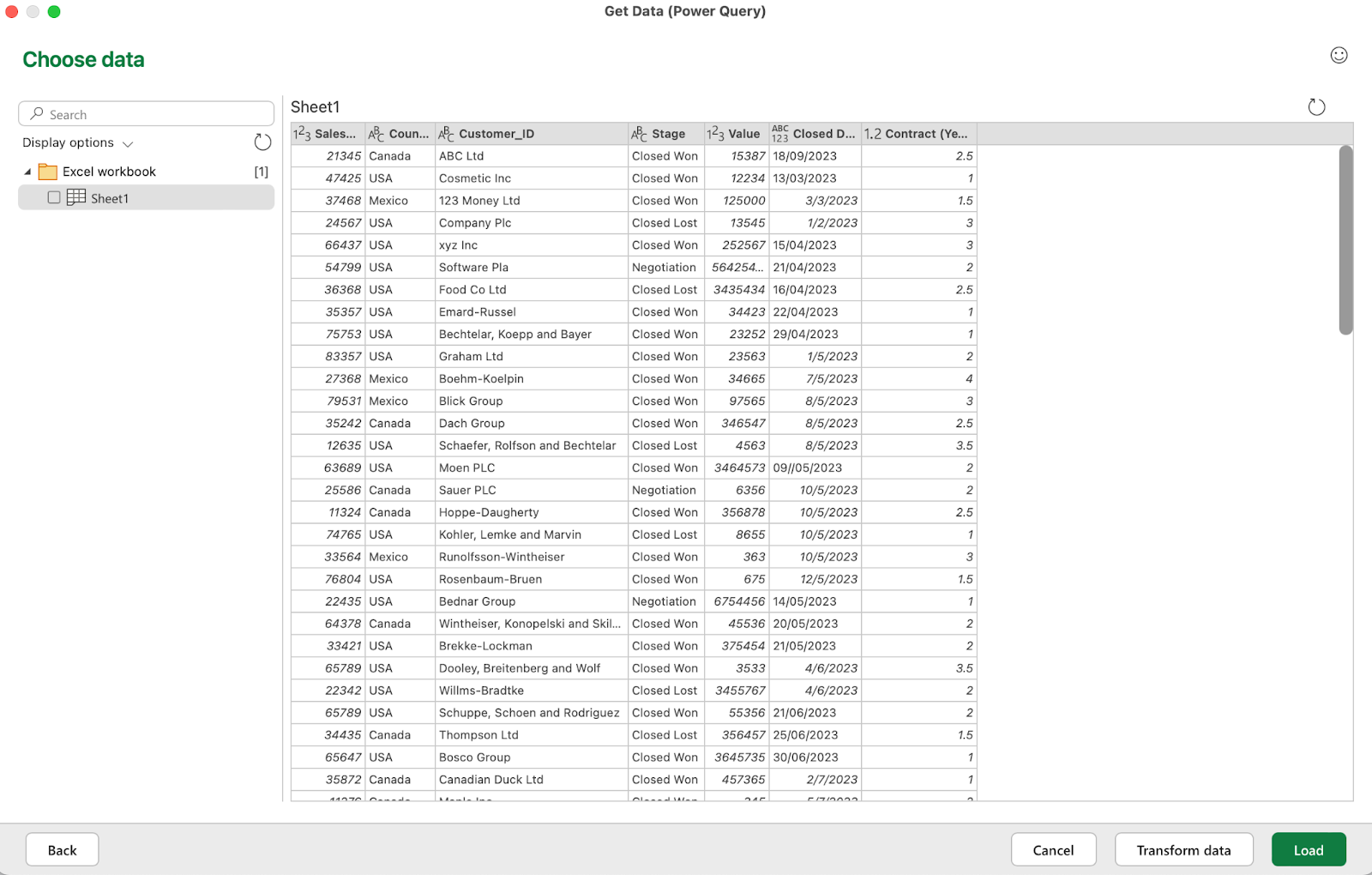
Clicking this option will open a window where you can choose a data source. As you’ll see, it’s possible to pull data from a wide range of sources, including shared SharePoint files.

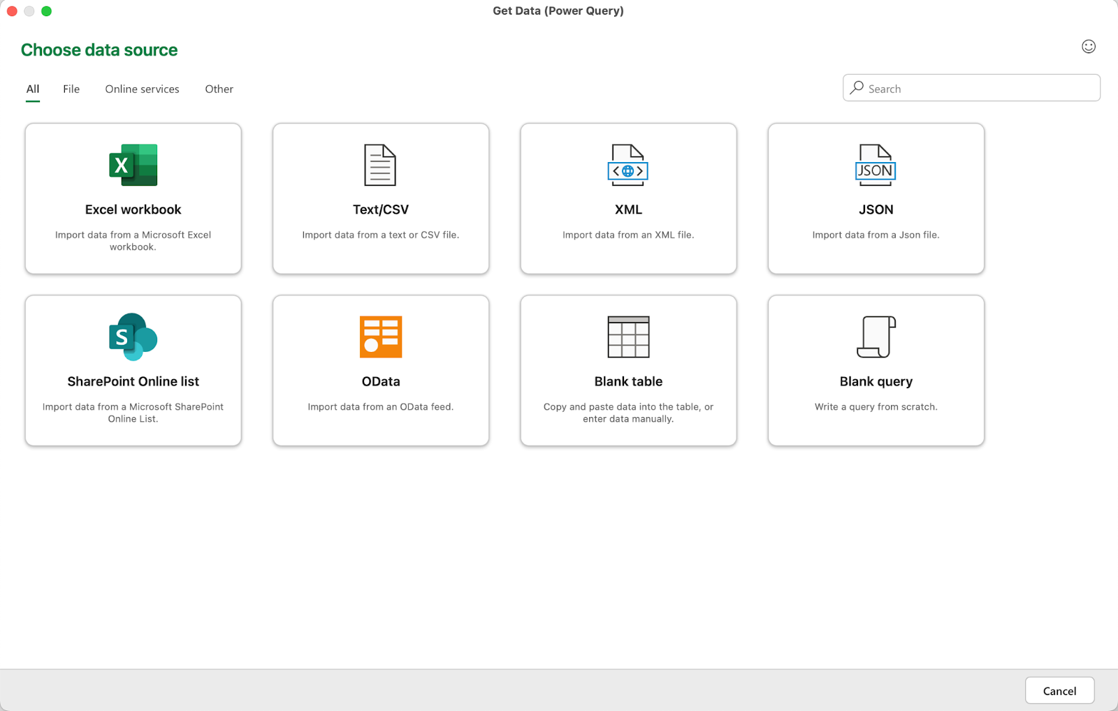
In this case, we’re selecting “Excel workbook” to access the file that is stored locally on my computer. After making this selection, you simply browse your files for the right spreadsheet and hit “Get Data.”

Then, on the following screen, hit “Next.” From here, you can select specific sheets that you want to import. You’ll be able to preview the data before hitting “Load” to finalize the import.

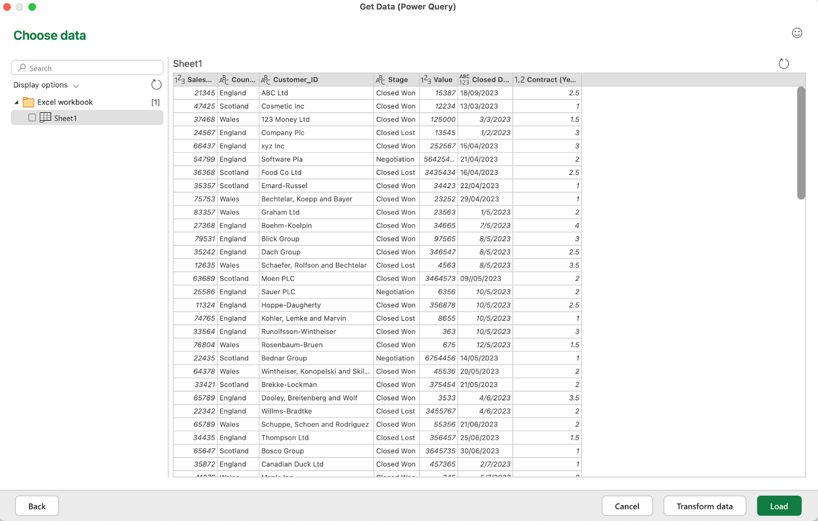
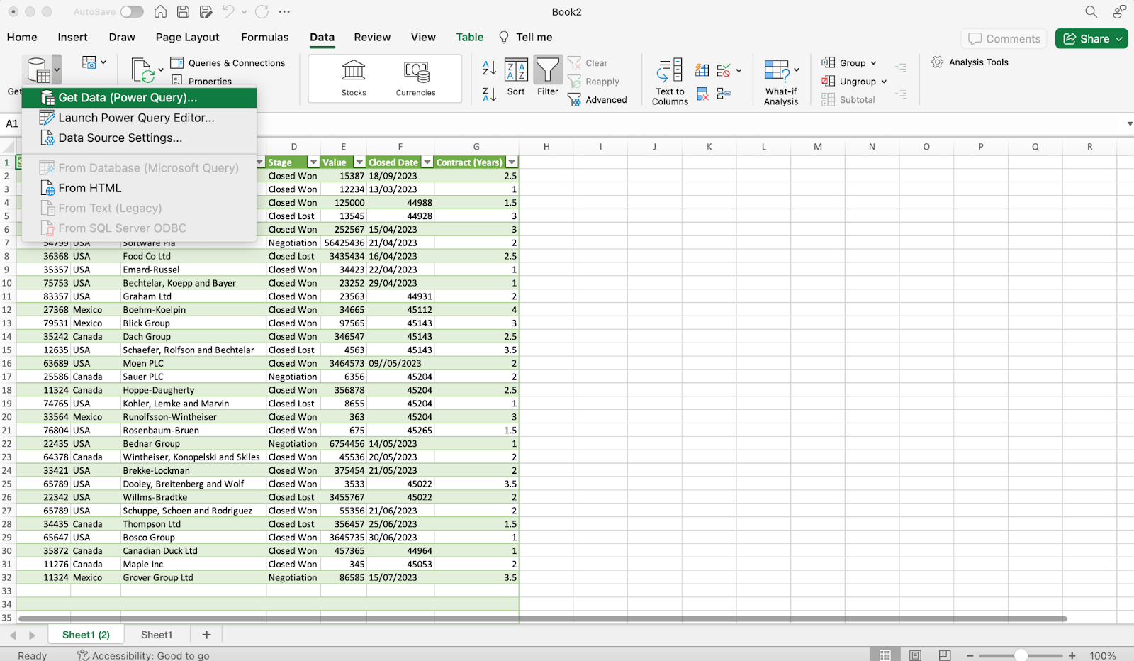
If you select “Load” at this stage, power query will import the data into a new tab on your existing spreadsheet.

From there, you can select “Data” and “Launch Power Query Editor” to perform mass cleaning or updating of the imported data.

Step 3. Cleaning imported data.

If you prefer to clean your data before you import it, you can do so during the import stage.

Instead of selecting “Load” during the import process, you can select “Transform data,” which opens the Power Query Editor just like in the previous step.

For instance, the U.K. sales sheet contains the same data as the U.S. sheet, but it’s not formatted correctly. The currency format is not applied to the currency cell.

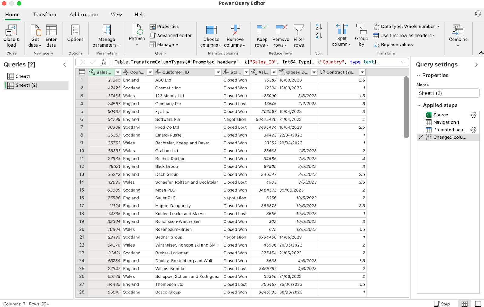
So, in Power Query Editor, I can select the “Transform” tab to edit the data before I import it (I could also do this if I imported the data first and then opened the Power Query Editor).

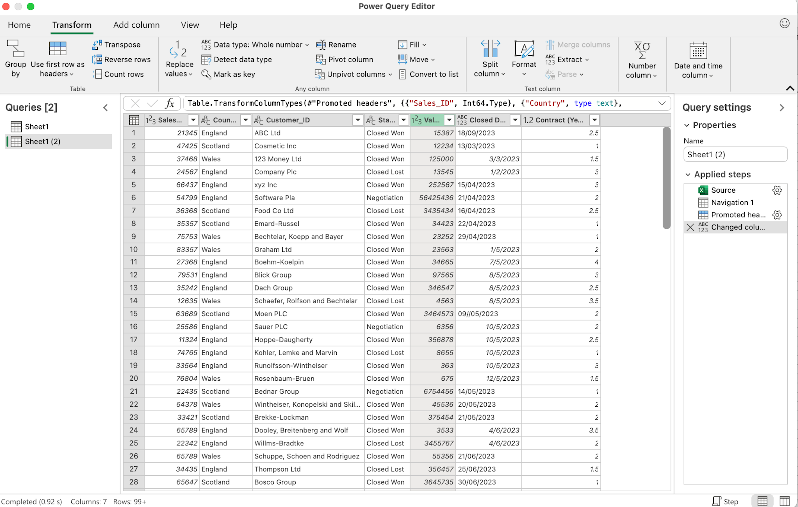
As you can see, there are tons of options available to you here. In this instance, I’m going to select the Currency column and selecting “Data type.”

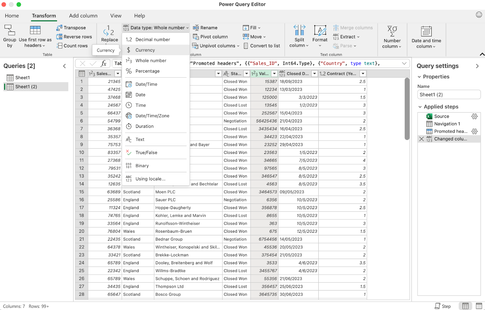
From there, I can select the Currency option and change the value to USD.

Step 4. Load your transformed data.

The final step is adding this cleaned and transformed data into my existing spreadsheet. In Power Query Editor, navigate back to the “Home” tab and click “Close & load.”

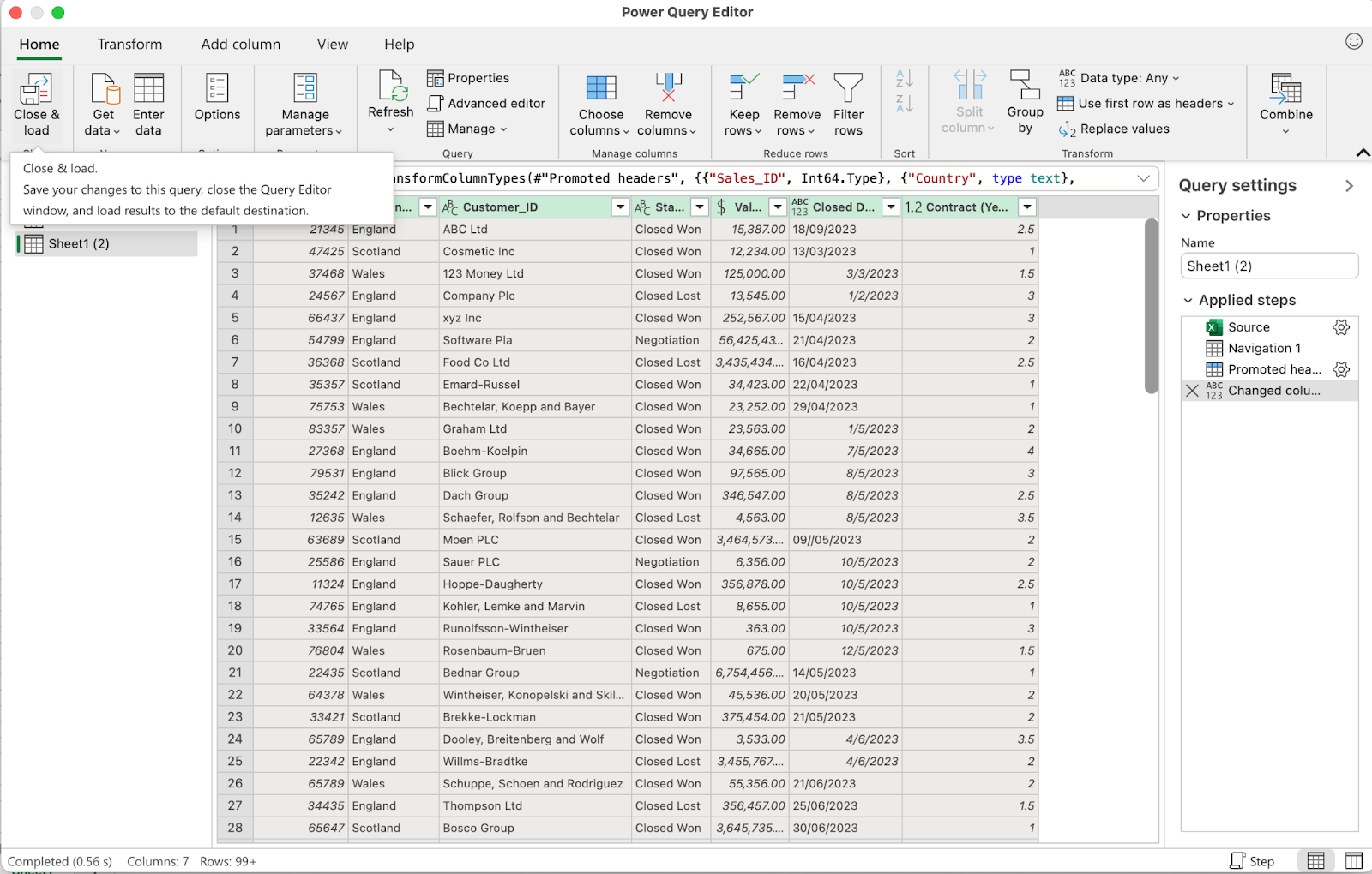
Excel will now load this query into a new tab on your spreadsheet.

This simple step-by-step process shows you how to get started with accessing and using power query.

The use cases for power query, however, are almost endless due to the wide variety of data you can import and clean, and the types of transformations and data manipulations you can perform.

So, let’s take a look at some examples of what you can use power query to do.

Power Query Examples

Consolidating Data From Multiple Spreadsheets

Whether you’re working with multiple workbooks of your own creation or having files sent your way from other people, the need to consolidate data into one sheet is a fairly common problem.

Power query makes this a pretty straightforward task.

First, make sure all the workbooks you want to consolidate are saved in the same folder. Where possible, make sure they all match in terms of having the same column headings.

Open up Excel to a blank workbook and access power query with the “Get Data” option.

Select your data source as “Excel workbook” and choose your first file. If your sheets are all formatted the same, you won’t need to do anything else here. Simply hit “Load.”

Next, you’re going to import your other spreadsheets. But, instead of performing this first step the exact same way, you’re going to append the other sheets to this existing query that you’ve just created.

In the sheet, open power query again and select the second workbook from your list when importing a file. Instead of hitting “Load,” select the “Transform Data” option.

Now, you should see both queries available in the Power Query Editor on the left side panel.

On the right-hand side of the ribbon in Power Query Editor, you’ll see a “Combine” button with a dropdown containing options to merge or append queries.

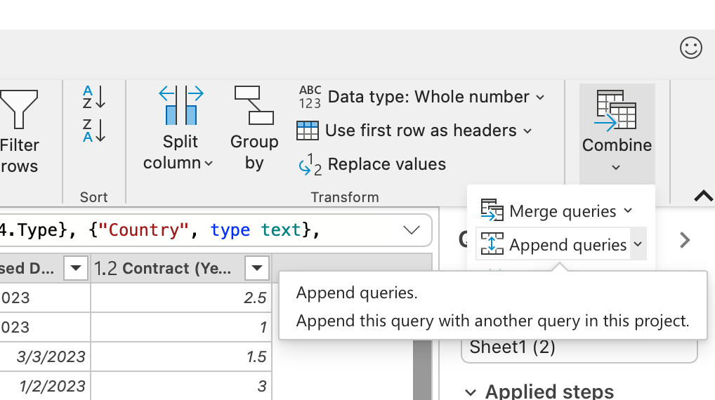
From the dropdown, select “Append queries as new.” Select the tables as you’d like to append one to the end of the other, and hit “Ok.”

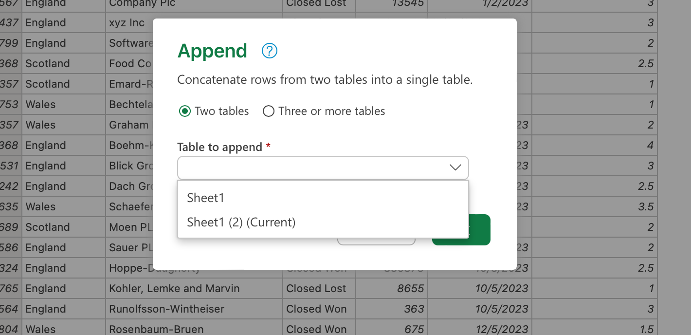
Power query will append the two tables together in one tab on your sheet. You can perform this action with two spreadsheets or multiple spreadsheets, depending on your needs.

Cleaning Up Data Before Importing

Sometimes, you can be dealing with a messy spreadsheet. Formatting and styling are all over the place, and you want to make sure it’s as clean and tidy as possible before importing.

Power query makes this an easy part of the process as you import data, so you don’t have to spend time manually cleaning things up afterward.

A simple example is a spreadsheet where some text is capitalized, and some is not. So, the goal is to convert everything into sentence case before adding it to your existing sheet.

Let’s say the sales team in France has sent us their sales report. It looks great, but some text in the Country ID column is in all caps, and some is not. Plus, random spaces have appeared in the country name that need to be fixed, too, or we’ll struggle to properly pull the data into pivot tables and other reporting.

In your sheet, open power query and import the file with the messy data. Click “Transform data” rather than importing it straight away.

First, find the column with the mixed-up capitalization and extra spaces. Right-click on the column and click “Transform column,” then “Text transforms” and, finally, “Trim.” This will remove any extra spacing that could interfere with manipulating the data.

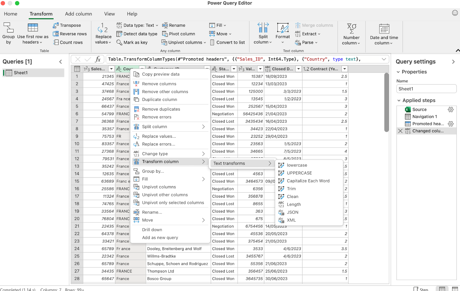
Right-click on the column again, and this time, click “Capitalize Each Word” from the options. You may need to first select “lowercase” to fix any All-Caps words and then use the “Capitalize Each Word” option.

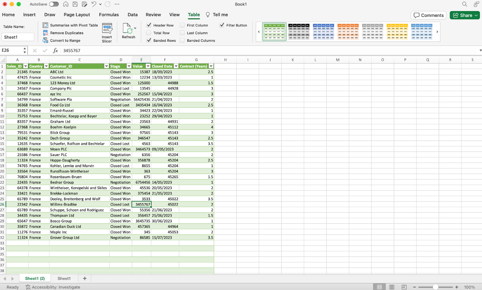
Now, you can click “Load” for your cleaned data to import into your Excel sheet.

Unpivoting/Pivoting Data to Improve Analysis Capabilities

Another common challenge with Excel is receiving data in a way that makes it difficult to manipulate and analyze, specifically when you want to switch around columns and rows — or “pivot” the data.

In this example, we have survey data where the columns are parsed out by respondents. Ideally, we’d like it parsed out with the columns as the survey questions.

First, open a blank Excel table and import your sheet using power query.

Like the previous example, instead of clicking “Load,” we first need to click “Transform data.”

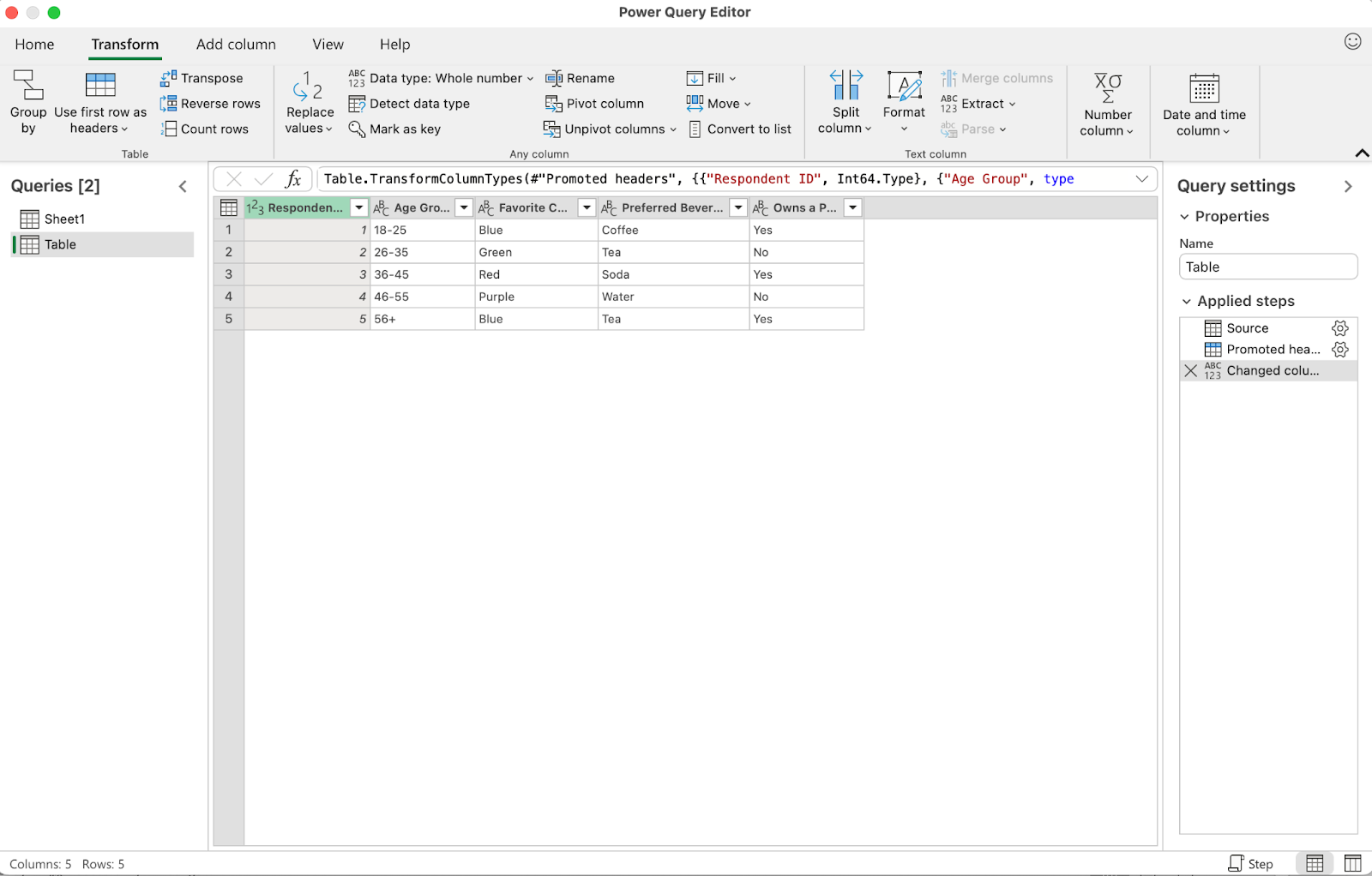
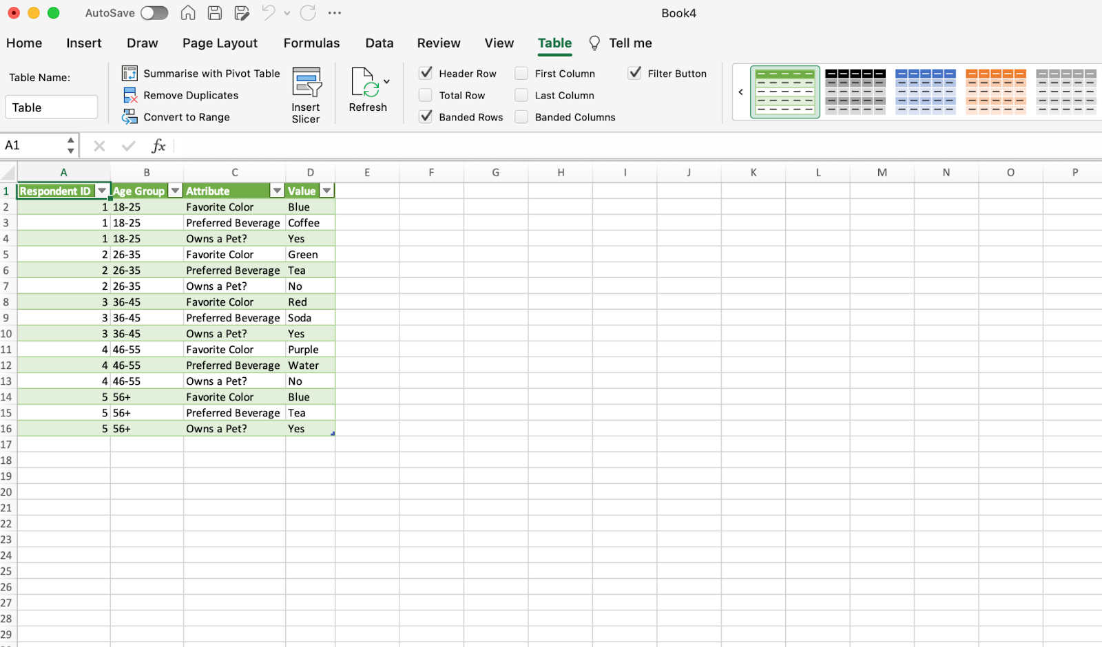
Now that Power Query Editor is open, navigate to the Transform tab in the ribbon. Select all the survey question columns together, and click “Unpivot columns” and then select “Unpivot only selected columns.”

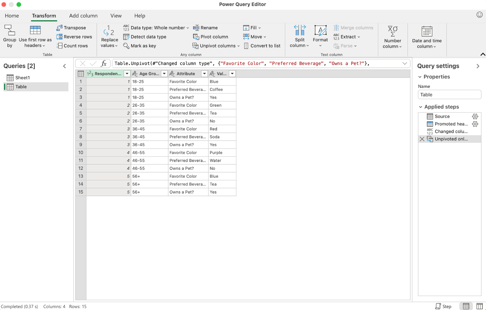
Power query takes the selected columns and parses out the data by the attributes and values of the questions. Navigate back to the “Home” tab and hit “Close & load” to use the unpivoted data in your spreadsheet.

Get Experimental With Power Query

In the grand scheme of tools, Excel is amongst the most powerful when it comes to sorting, cleaning, and transforming the type of data that gets used in day-to-day business operations across multiple departments and teams.

While it can take a little while to get familiar with all the features and functionalities of something like power query, it’s well worth the effort.

Even with relatively simple spreadsheets that just contain a lot of data, power query can cut your cleaning and transforming time down significantly, so you can get into important analysis and decision-making much quicker.